Multiscale modeling in biology

Multiscale modeling in biology is used to take into account the complex interactions between the different organization levels in living systems. We review several models, from the most simple to the complex ones, and discuss their properties from a multiscale point of view.

Last edited: 06/01/2013

http://sfbt-2012.imag.fr http://math.univ-lyon1.fr/~bernard/index.php?texte=SFBT

Download the M-files

Lotka-Volterra Equations (1925)
FKPP Equation (1937)
Turing Equations (1952)
Keller-Segel Equations (1970)
Langevin and Fokker-Planck Equations
Hoffman et al. (2008)

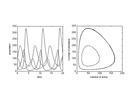
Lotka-Volterra Equations (1925)

We begin with the classic Lotka-Volterra predator-prey model

x' = x * (a - b * y)

y' = -y * (c - d * x)

The variables x and y measure the sizes of the prey and predator populations respectively. The interpretation at the population scale is the following: the growth rate of the the prey population is constant (a * x) and the death rate of the preys is proportional to the number of predators (b * y * x).

To simulate a system, we use the function called LOTKAVOLTERRA

type lotkavolterra

function xxp = lotkavolterra(~,xx)
% LOTKAVOLTERRA Predator-prey Lotka-Volterra system
%
%   Examples
%       sol1 = ode23(@lotkavolterra,[0 20],[ 20 20 ]);
%       sol2 = ode23(@lotkavolterra,[0 20],[ 100 100 ]);
%       xint = linspace(0,20,500); 
%       yint1 = deval(sol1,xint); yint2 = deval(sol2,xint);
%       subplot(121)
%       plot(xint,yint1,'LineW',1,'Color','k'); hold on
%       plot(xint,yint2,'LineW',2,'Color',[0.6 0.6 0.6])
%       axis square
%       xlabel('time'); ylabel('population'); 
%       subplot(122)
%       plot(yint1(1,:),yint1(2,:),'LineW',1,'Color','k'); hold on
%       plot(yint2(1,:),yint2(2,:),'LineW',2,'Color',[0.6 0.6 0.6])
%       axis square
%       xlabel('number of preys'); ylabel('number of predators'); 
%
%   See also
%
%   Ecole de Printemps SFBT 2012

x = xx(1); y = xx(2);
a = 1; b = 0.01;
c = 1; d = 0.02;

xxp = [ x * (a - b * y)
     -y * (c - d * x)];

We solve the Lotka-Volterra system for times between 0 and 50, using the ode23 solver.

sol1 = ode23(@lotkavolterra,[0 20],[ 20 20 ]);
sol2 = ode23(@lotkavolterra,[0 20],[ 100 100 ]);

Plot the result of the simulation two different ways.

xint = linspace(0,20,500);
yint1 = deval(sol1,xint); yint2 = deval(sol2,xint);
subplot(121)
plot(xint,yint1,'LineW',1,'Color','k'); hold on
plot(xint,yint2,'LineW',2,'Color',[0.6 0.6 0.6])
axis square
xlabel('time'); ylabel('population');
subplot(122)
plot(yint1(1,:),yint1(2,:),'LineW',1,'Color','k'); hold on
plot(yint2(1,:),yint2(2,:),'LineW',2,'Color',[0.6 0.6 0.6])
axis square
xlabel('number of preys'); ylabel('number of predators');

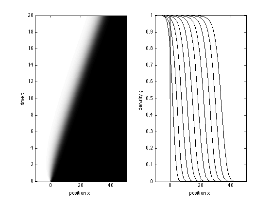
FKPP Equation (1937)

The Fisher-Kolmogorov-Petrovskii-Piskunov (FKPP) equation is a reaction-diffusion partial differential equation. It was introduced by R.A. Fisher in 1937 as a model for the spread of an advantageous gene in a population.

\rho_t = D \rho_{xx} + r \rho (1 - \rho)

The equation describes the frequency rho(t,x) of the advantageous gene in a population located at position x, at time t.

To simulate the equation, we use the functions fkpp and fkppbc.

type fkpp
type fkppbc

function [c,f,s] = fkpp(x,t,u,DuDx)
% FKPP PDE components for the FKPP equation
%
%   Examples
%       x = -10:0.1:50;
%       t = 0:0.1:20;
%       sol = pdepe(0,@fkpp,@(x) (x<=0),@fkppbc,x,t);
%       u1 = sol(:,:,1);
%       imagesc(x,t,u1); axis xy;
%       colormap gray
%       xlabel('position x'); ylabel('time t')
%
%       plot(x,u1(1,:),'LineW',2,'Color',[0.6 0.6 0.6]) % initial condition
%       hold on 
%       plot(x,u1(21:20:201,:),'k')
%       axis tight
%       xlabel('position x'); ylabel('density \rho')
%
%   See also: FKPPBC, PDEPE
%
%   Ecole de Printemps SFBT 2012   

r = 1; D = 1;

c = 1;
f = D * DuDx;
s = r * u .* (1 - u);

function [pl,ql,pr,qr] = fkppbc(xl,ul,xr,ur,t)
% FKPPBC Boundary condition for the FKPP equation
%
%   See also: FKPP
%
%   Ecole de Printemps SFBT 2012   

pl = 0; pr = 0;
ql = 1; qr = 1;

We solve the FKPP equation for times between 0 and 20 and space between -10 and 50, with an initial condition equal to one if x<=0 and zero otherwise

(x<=0)

using the PDE solve PDEPE

x = -10:0.1:50;
t = 0:0.1:20;
sol = pdepe(0,@fkpp,@(x) (x<=0),@fkppbc,x,t);
u1 = sol(:,:,1);

Plot the result of the simulation two different ways.

figure(2)
subplot(121)
imagesc(x,t,u1); axis xy;
colormap gray
xlabel('position x'); ylabel('time t')
view(2)
axis tight
subplot(122)
plot(x,u1(1,:),'LineW',2,'Color',[0.6 0.6 0.6]) % initial condition
hold on
plot(x,u1(21:20:201,:),'k')
axis tight
xlabel('position x'); ylabel('density \rho')

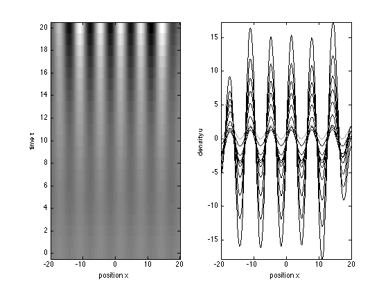
Turing Equations (1952)

Alan M. Turing introduced this famous system in 1952 to show how spatial patterns (spatially heterogeneous solutions) could arise from diffusion of chemical substances. One morphogen is an activator and the other one is an inhibitor. The activator, u activates itself with a rate fu and activates the inhibitor with a rate gu. The inhibitor, v, inhibits itself with a rate gv and inhibits the activator with a rate fv. If the diffusion rate of the activator is much smaller than the diffusion rate of the inhibitor, the concentrations of u and v can show spatial instabilities.

u_t = D_u u_{xx} + fu * u + fv * v

v_t = D_v v_{xx} + gu * u + gv * v

To simulate the equations, we use the functions turing, turingbc and turingic

type turing
type turingbc
type turingic

function [c,f,s] = turing(x,t,u,DuDx)
% TURING PDE components for the Turing equations
%
%   Examples
%       x = -20:0.1:20;
%       t = 0:20;
%       sol = pdepe(0,@turing,@turingic,@turingbc,x,t);
%       u = sol(:,:,1);
%       v = sol(:,:,2);
%       imagesc(x,t,u); axis xy;
%       colormap gray
%       xlabel('position x'); ylabel('time t')
%
%       plot(x,u(1,:),'Color',[0.6 0.6 0.6],'LineW',1.5) % initial condition
%       hold on 
%       %plot(x,v(1,:),'--','LineW',1.5) % initial condition 
%       plot(x,u(3:2:20,:),'k')
%       %plot(x,u(3:2:20,:),'--k')
%       axis tight
%       xlabel('position x'); ylabel('density u')
%
%   See also: TURINGIC, TURINGBC, PDEPE
%
%   Ecole de Printemps SFBT 2012   

fu = 0.4; fv = -0.5;
gu = 1; gv = -0.5;
f1 = fu * u(1) + fv * u(2);
f2 = gu * u(1) + gv * u(2);
Du = 0.2; Dv = 10;

c = [1 1]';
f = [Du 0; 0 Dv] * DuDx;
s = [f1 f2]';

function [pl,ql,pr,qr] = turingbc(xl,ul,xr,ur,t)
% TURINGBC Boundary conditions for Turing equations
%
%   See also: TURING, TURINGIC
%
%   Ecole de Printemps SFBT 2012 

pl = [0 0]'; pr = [0 0]';
ql = [1 1]'; qr = [1 1]';

function u0 = turingic(x)
% TURINGIC Initial conditions for Turing equations
%
%   See also: TURING, TURINGBC
%
%   Ecole de Printemps SFBT 2012 

u0 = [1+sin(x); 1+cos(x)];

We solve the Turing equations for times between 0 and 20 and space between -20 and 20, with an initial condition given by the function turingic

x = -20:0.1:20;
t = 0:20;
sol = pdepe(0,@turing,@turingic,@turingbc,x,t);
u = sol(:,:,1);
v = sol(:,:,2);

Plot the result of the simulation two different ways.

figure(3)
subplot(121)
imagesc(x,t,u); axis xy;
colormap gray
xlabel('position x'); ylabel('time t')
subplot(122)
plot(x,u(1,:),'Color',[0.6 0.6 0.6],'LineW',1.5) % initial condition
hold on
plot(x,u(3:2:20,:),'k')
axis tight
xlabel('position x'); ylabel('density u')

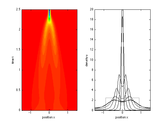
Keller-Segel Equations (1970)

Chemotaxis is the phenomenon in which cells move according to the concentration of certain molecules in the environment. They could be attracted by food, or repelled by poisons. If the cells themselves secrete the chemotactic molecules, we can describe the movement of the cells by the celebrated Keller-Segelmodel.

u_t = d u_{xx} - (u * v)_x

v_t = epsilon * v_{xx} + u - a * v

To simulate the equations, we use the functions kellersegel , kellersegelbc and kellersegelic.

type kellersegel
type kellersegelbc
type kellersegelic

function [c,f,s] = kellersegel(~,~,u,DuDx)
% KELLERSEGEL PDE components for Keller-Segel equations
%
%   Examples
%       x = -1.5:0.01:1.5;
%       t = 0:0.01:2.5;
%       sol = pdepe(0,@kellersegel,@kellersegelic,@kellersegelbc,x,t);
%       u = sol(:,:,1);
%       v = sol(:,:,2);
%       imagesc(x,t,u); axis xy;
%       colormap hsv
%       xlabel('position x'); ylabel('time t')
%
%       plot(x,u(1,:),'Color',[0.6 0.6 0.6],'LineW',1.5) % initial condition
%       hold on 
%       plot(x,u([26 51 101 151 201 226 251],:),'k')
%       axis([-1.5 1.5 0 20])
%       xlabel('position x'); ylabel('density u')
%
%
%   See also: KELLERSEGELIC, KELLERSEGELBC, PDEPE
%
%   Ecole de Printemps SFBT 2012

a = 0.1;
f1 = 0;
f2 = u(1) - a * u(2);
d = 0.5; epsilon = 0.05; %0.01

c = [1 1]';
f = [d, -u(1); 0 epsilon] * DuDx;
s = [f1 f2]';

function [pl,ql,pr,qr] = kellersegelbc(xl,ul,xr,ur,t)
% KELLERSEGELBC Boundary conditions for Keller-Segel equations
%
%   See also: KELLERSEGEL, KELLERSEGELIC
%
%   Ecole de Printemps SFBT 2012

pl = [0 0]'; pr = [0 0]'; 
ql = [1 1]'; qr = [1 1]';

function u0 = kellersegelic(x)
% KELLERSEGELIC Initial conditions for Keller-Segel equations
%
%   See also: KELLERSEGEL, KELLERSEGELBC
%
%   Ecole de Printemps SFBT 2012

c = 0.5;
d = 0.4;
u0 = [1/d*(x>=-c-d).*(x<=-c+d)+1/d*(x>=c-d).*(x<=c+d); 0];

We solve the Keller-Segel equations for times between 0 and 2.5 and space between -2 and 2, with an initial condition equal to one between x = -1 and x = 1

x = -1.5:0.01:1.5;
t = 0:0.01:2.5;
sol = pdepe(0,@kellersegel,@kellersegelic,@kellersegelbc,x,t);
u = sol(:,:,1);
v = sol(:,:,2);

Plot the result of the simulation two different ways.

figure(4)
subplot(121)
imagesc(x,t,u); axis xy;
colormap hsv
xlabel('position x'); ylabel('time t')
subplot(122)
plot(x,u(1,:),'Color',[0.6 0.6 0.6],'LineW',1.5) % initial condition
hold on
plot(x,u([26 51 101 151 201 226 251],:),'k')
axis([-1.5 1.5 0 20])
xlabel('position x'); ylabel('density u')

Langevin and Fokker-Planck Equations

The nonlinear Langevin equation is

y' = f(y) + g(y) * xi(t)

where xi(t) is a Gaussian, uncorrelated noise. We look at the example of the Lotka-Volterra equations

x' = x * (a - b * y) + e*xi_x

y' = -y * (c - d * x) + f*xi_y

To simulate the equations, we use the function sdeEuler

type sdeEuler

function [t,y]=sdeEuler(f,tspan,ic,sdnoise,varargin)
% SDEEULER Stochastic Differential Equation solver with the Euler method
%
%   Examples
%       Solve the equation y'(t) = -0.1*y(t) + 0.1*xi(t)
%       with IC y(0)=1, with 10 realizations
%       [t, y] = sdeEuler(@(t,y) -0.1*y, [0 10],ones(1,10),0.1*ones(1,10));
%       plot(t,y,'k','LineW',0.5); axis tight
%       xlabel('time t'); ylabel('y(t)')
%
%       [t1, y1] = sdeEuler(@lotkavolterra, [0 60],[20 20]',3*ones(2,1));
%       [t2, y2] = sdeEuler(@lotkavolterra, [0 60],[100 100]',3*ones(2,1));
%       clf;
%       subplot(121)
%       plot(t1,y1,'LineW',1,'Color','k'); hold on
%       plot(t2,y2,'LineW',1,'Color',[0.6 0.6 0.6])
%       axis square
%       xlabel('time'); ylabel('population'); 
%       subplot(122)
%       plot(y1(1,:),y1(2,:),'LineW',1,'Color','k'); hold on
%       plot(y2(1,:),y2(2,:),'LineW',1,'Color',[0.6 0.6 0.6])
%       axis square
%       xlabel('number of preys'); ylabel('number of predators'); 
%
%   Ecole de Printemps SFBT 2012

h=.01;
sh=sqrt(h);
t=tspan(1):h:tspan(2);
y=zeros(length(ic),length(t));
y(:,1)=ic;
stopcond=false;
for i=1:length(t)-1,
    y(:,i+1)=y(:,i)+h*feval(f,t,y(:,i),varargin{:})+sh*sdnoise.*randn(size(sdnoise));
    if stopcond && any(y(:,i+1)<0)
        yz =find(y(:,i+1)<0);
        y(yz,i+1)=0;
        sdnoise(yz)=0;
    end
end

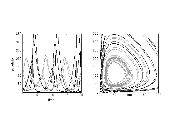
We solve the Langevin equations, with initial condition [x0,y0]'=[20 20]' and [x0,y0]'=[100 100]', with e=f=3.

[t1, y1] = sdeEuler(@lotkavolterra, [0 60],[20 20]',3*ones(2,1));
[t2, y2] = sdeEuler(@lotkavolterra, [0 60],[100 100]',3*ones(2,1));

Plot the solutions of the Langevin equation

figure(5)
subplot(121)
plot(t1,y1,'LineW',1,'Color','k'); hold on
plot(t2,y2,'LineW',1,'Color',[0.6 0.6 0.6])
axis([0 20 0 350])
axis square
xlabel('time'); ylabel('population');
subplot(122)
plot(y1(1,:),y1(2,:),'LineW',1,'Color','k'); hold on
plot(y2(1,:),y2(2,:),'LineW',1,'Color',[0.6 0.6 0.6])
axis([0 200 0 350])
axis square
xlabel('number of preys'); ylabel('number of predators');

The Fokker-Planck equation is

p_t = - (f(y) * p)_y + 1/2 * (g(y)^2 p)_{yy}

Compare Langevin and Fokker-Planck equations. We use the functions fokkerplanck and fokkerplanckbc

type fokkerplanck
type fokkerplanckbc

function [c,f,s] = fokkerplanck(x,t,u,DuDx)
% FOKKERPLANCK PDE components for the Fokker-Planck equation
%
%   Examples
%       x = -1:0.1:1.2;
%       t = 0:0.1:30;
%       sol = pdepe(0,@fokkerplanck,@(x) 10*(x>=1).*(x<=1.1),@fokkerplanckbc,x,t);
%       u1 = sol(:,:,1);
%       surf(x,t,u1);
%
%   See also: FOKKERPLANCKBC, PDEPE
%
%   Ecole de Printemps SFBT 2012   

r = 0.1; D = 0.5 * (0.1)^2;

c = 1;
f = D * DuDx + r * x * u;
s = 0;

function [pl,ql,pr,qr] = fokkerplanckbc(xl,ul,xr,ur,t)
% FOKKERPLANCKBC Boundary condition for the Fokker-Planck equation
%
%   See also: FOKKERPLANCKBC
%
%   Ecole de Printemps SFBT 2012   

pl = 0; pr = 0;
ql = 1; qr = 1;

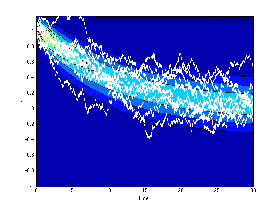
We solve the Fokker-Planck equation corresponding to the Langevin equation y' = -0.1 (y + xi), with initial conditions uniform between y=1 and y=1.1, for t=[0,30].

y = -1:0.1:1.2;
t = 0:0.1:30;
sol = pdepe(0,@fokkerplanck,@(y) 10*(y>=1).*(y<=1.1),@fokkerplanckbc,y,t);
u1 = sol(:,:,1);

We solve the Langevin eqaution 10 times for t=[0,30], with random initial conditions distributed uniformly between y=1.0 ans y=1.1

iclangevin = rand(10,1)/10+1.0;
[tl, yl] = sdeEuler(@(t,y) -0.1*y, [0 30],iclangevin,0.1*ones(10,1));

We plot and compare the solution of the Fokker-Planck equation and the solutions of the Langevin equation.

figure(6); clf
contourf(t,y,u1');
hold on
plot(tl,yl,'w')
xlabel('time')
ylabel('y')

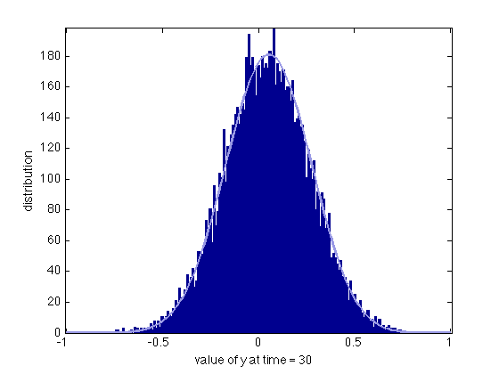
We compare the histogram of 10000 realizations of the Langevin equation at time t=30 with the solution of the Fokker-Planck equation.

runNb = 1e4;
iclangevin = rand(runNb,1)/10+1.0;
[tl, yl] = sdeEuler(@(t,y) -0.1*y, [0 30],iclangevin,0.1*ones(runNb,1));

figure(7); clf;
binWidth = 0.01;
bins = -1:binWidth:1;
hist(yl(:,end),bins)
hold on
u1normalized = runNb*binWidth*u1(end,:)/trapz(y,u1(end,:));
u1int = interp1(y,u1normalized,bins,'spline')';
plot(bins,u1int,'LineWidth',2,'Color',[0.6 0.6 0.9])
axis tight
set(gca,'FontS',14)
xlabel('value of y at time = 30');
ylabel('distribution')
clear y1

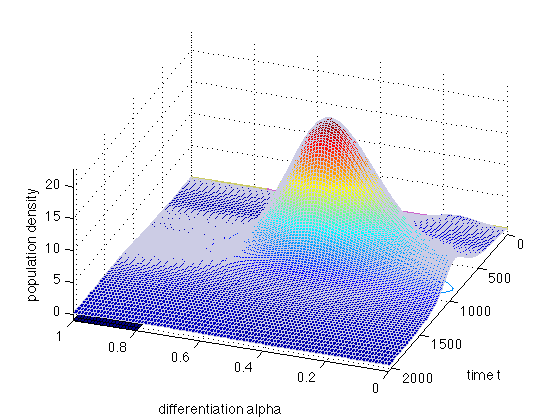
Hoffman et al. (2008)

Hoffmann and colleagues considered a model in which cell differentiate by moving randomly into a differentiation space.

% To simulate the equations, we use the functions hoffFK and hoffFKbc

type hoffFK
type hoffFKbc

function [c,f,s] = hoffFK(x,t,u,DuDx,par)
% HOFFFK PDE components for the Hoffmann et al. equation
%
%   Example 1
%       No differentiation, only proliferation
%       ** Set r0 = 0 and r1 = 0 **
%       x = [0 0.05 0.09:0.01:0.21 0.25:0.05:1];
%       t = linspace(0,200,10);
%       mypde = @(x,t,u,DuDx) hoffFK(x,t,u,DuDx,[0 0]);
%       myic  = @(x) (x>=0.1).*(x<=0.2);
%       sol = pdepe(0,mypde,myic,@hoffFKbc,x,t);
%       u1 = sol(:,:,1);
%       surfc(x,t,u1,'LineStyle','none');
%
%   Example 2
%       Differentiation and proliferation
%       ** Set r0 = 0.01 and r1 = 0.5 **
%       x = 0:0.1:1;
%       t = linspace(0,200,10);
%       mypde = @(x,t,u,DuDx) hoffFK(x,t,u,DuDx,[0.01 0.05]);
%       myic  = @(x) (x>=0.1).*(x<=0.2);
%       sol = pdepe(0,mypde,myic,@hoffFKbc,x,t);
%       u1 = sol(:,:,1);
%       surfc(x,t,u1);
%
%   See also: HOFFFKBC, PDEPE
%
%   Ecole de Printemps SFBT 2012

maxProlif = 0.02;
r0 = par(1);
r1 = par(2);
maxNoise = 0.2;
minNoise = 0.1;

c = 1;
f = 0.5*(differentiation(x).*sigma2(x).*DuDx + ...
    (differentiation(x).*ds2(x)+ddr(x).*sigma2(x)).*u);
s = prolif(x)*u;

    function y = prolif(x)
        % PROLIF is the proliferation rate of x-cells        
        y = 4*maxProlif*x.*(1-x); 
    end

    function y = differentiation(x)
        % DIFFERENTIATION is the differentiation rate of x-cells     
        y = r0 + r1*prolif(x);
    end

    function y = ddr(x)
        % DDR derivative of DIFFERENTIATION
        % Used to compute f
        y = r1*4*maxProlif*(1-2*x);
    end

    function y = sigma2(x)
        % SIGMA2 differentiation noise
        y = minNoise + 4*maxNoise*(x-0.5).^2;
    end

    function y = ds2(x)
        % DS2 derivative of SIGMA2
        % Used to compute f
        y = 8*maxNoise*(x-0.5);
    end
end


function [pl,ql,pr,qr] = hoffFKbc(xl,ul,xr,ur,t)
%HOFFFKBC Boundary condition for the Hoffmann et al. equation
%
%   See also: HOFFFK
%
%   Ecole de Printemps SFBT 2012   

pl = 0; pr = 0;
ql = 1; qr = 1;

We solve the Hoffmann equation for t=[0,200] and space x=[0,1], with an initial condition equal to one for x=[0.1,0.2].

In the first example, we solve the equation when there is no differentiation: R(alpha)=0. Set r0=0.0 and r1=0.0.

x = [0 0.05 0.09:0.01:0.21 0.25:0.05:1];
t = linspace(0,200,10);
mypde = @(x,t,u,DuDx) hoffFK(x,t,u,DuDx,[0 0]);
myic  = @(x) (x>=0.1).*(x<=0.2);
sol = pdepe(0,mypde,myic,@hoffFKbc,x,t);
u1 = sol(:,:,1);

figure(8); clf;
surfc(x,t,u1,'EdgeColor',[0.4 0.4 0.4]);

set(gca,'FontS',14);
xlabel('differentiation alpha');
ylabel('time t');
zlabel('population density')
view(-159.5,44);
hold on
plot3(x,0*x,4*8*x.*(1-x),'LineWidth',2,'Color',[0.8 0.4 0.4])

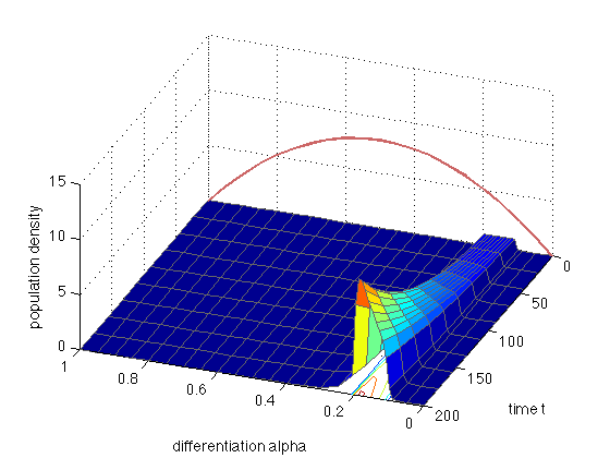
The red curve is the proliferation rate r(alpha) (in arbitrary units).

In the second example, we solve the equation when there is differentiation: R(alpha)=r0+r1*r(alpha). Set r0 = 0.01 and r1= 0.05.

x = 0:0.1:1;
t = linspace(0,200,10);
mypde = @(x,t,u,DuDx) hoffFK(x,t,u,DuDx,[0.01 0.05]);
myic  = @(x) (x>=0.1).*(x<=0.2);
sol = pdepe(0,mypde,myic,@hoffFKbc,x,t);
u1 = sol(:,:,1);

figure(9); clf;
surfc(x,t,u1,'EdgeColor',[0.4 0.4 0.4]);

set(gca,'FontS',14);
xlabel('differentiation alpha');
ylabel('time t');
zlabel('population density')
view(-159.5,44);
hold on
plot3(x,0*x,4*4*x.*(1-x),'LineWidth',2,'Color',[0.8 0.4 0.4])
plot3(x,0*x,0.01+0.5*4*4*x.*(1-x),'LineWidth',2,'Color',[0.8 0.4 0.8])
plot3(x,0*x,0.1 + 4*3*(x-0.5).^2,'LineWidth',2,'Color',[0.8 0.8 0.4])

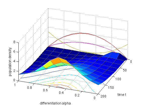
The red curve is the proliferation rate r(alpha). The green curve is the noise sigma2(alpha) and the blue curve is the differentiation rate R(alpha) (all in arbitrary units).

In the third example, we solve the equation with a growth limited by the total population.

% To simulate the equations, we use the function |mscelldiff|

help mscelldiff

  MSCELLDIFF Nonlinear PDE with population-dependent growth
   MSCELLDIFF solve the modified Fokker-Planck equation adapted from
   Hoffmann et al. (2008). The PDE is
 
      [1] *  D_ [u] =  D_ [0.5*(R*s2*DuDx+(R*ds2+dR*s2)*u)] + [r(x)*u*(1-NA/K)]
             Dt        Dx
      ----      ---       ---------------------------------   ---------
       c         u        f(x,t,u,Du/Dx)                      s(x,t,u,Du/Dx)
 
    where
        x           differentiation level x in [0,1]
        t           time
        u  = u(t,x) cell density at differentiation level x
        R  = R(x)   differentiation rate
        dR = dR(x)  derivative of the differentiation rate
        s2 = s2(x)  variance of the differentiation jumps
        ds2= ds2(x) derivative of s2
        r  = r(x)   proliferation rate
        NA =        cell population acting on the feedback
        K  =        carrying capacity
 
    Ecole de Printemps SFBT 2012

    Published output in the Help browser
       showdemo mscelldiff

We run the system with default parameters

figure(10); clf;
mscelldiff;

--------------------------------------------------
*******************************************

Multiscale modeling in biology

Contents

Lotka-Volterra Equations (1925)

FKPP Equation (1937)

Turing Equations (1952)

Keller-Segel Equations (1970)

Langevin and Fokker-Planck Equations

Hoffman et al. (2008)