Inferring Model Parameters in System Biology

Dataset with \(n\) observations \(y_i\) at time points \(t_i\), \(i=1,...,n\), and a model function \(m(t; \theta)\) that depends on time and on a certain number of parameters \(\theta = (\theta_1, \theta_2, \theta_k)\). Can we find values for \(\theta\) such that the function \(m\) will take values close to \(y_i\) when evaluated at \(t_i\):

\[ m(t_i; \theta) \sim y_i \]

Data

How to choose the model

If the number of parameter \(k\) equal to or larger than \(n\), it is in general possible to match exactly all the data: \(m_i = y_i\). This is called interpolation.

When the number of parameters if smaller than \(n\), it will be in general not possible to match all data points, and there will be a trade-off to achieve between being far-off for few data points and close to the others, or being a bit further away from all data point.

The way to resolve this trade-off is to pose a minimization problem. That is, we will define a scalar-valued objective-function \(f\) that depends on \(m\) and \(y\) and has the property that \(f(y,y) = 0\). By far the most common objective-function used in biology is the sum of squares of the error between \(m_i\) and \(y_i\): \[ f(m,y) = \sum_{i=1}^n (m_i - y_i)^2 = ||m - y||^2 \]

Small is beautiful

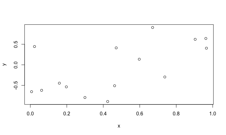
We randomly generate n=15 pairs of points, \(x\) in [0,1] and \(y\) in [-1,1].

n <- 15
x <- runif(n) # generate n random numbers in [0,1]
y <- runif(n, min = -1, 1) # generate response in [-1,1]
plot(x,y)

raw data

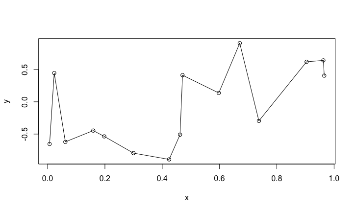
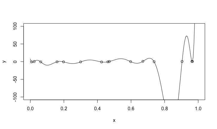
Polynomial interpolation

Now we fit a polynomial of degree 14 (it has 15 coefficients/parameters)

interp <- lm(y ~ poly(x,n-1))
    plot(x,y)
    sx <- sort(x)
    lines(sx, predict(interp, data.frame(x = sx)))

interpolated data

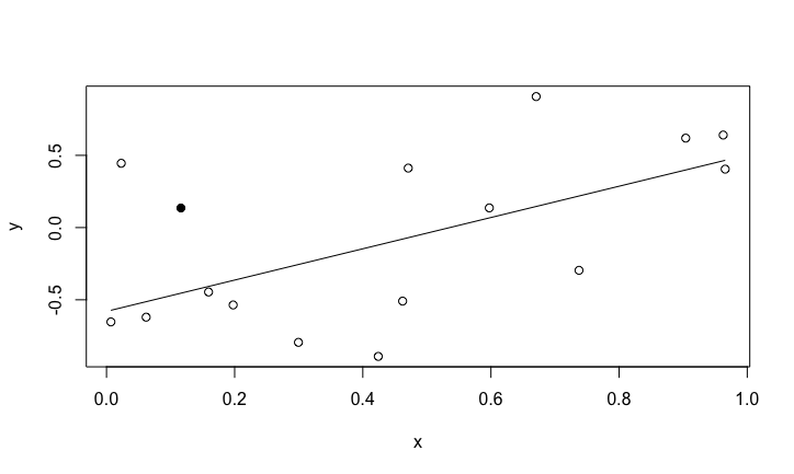
The fit is perfect, the polynomial function goes through all the data points. Suppose we get a new pair of data \((x,y)\). How good will be the prediction?

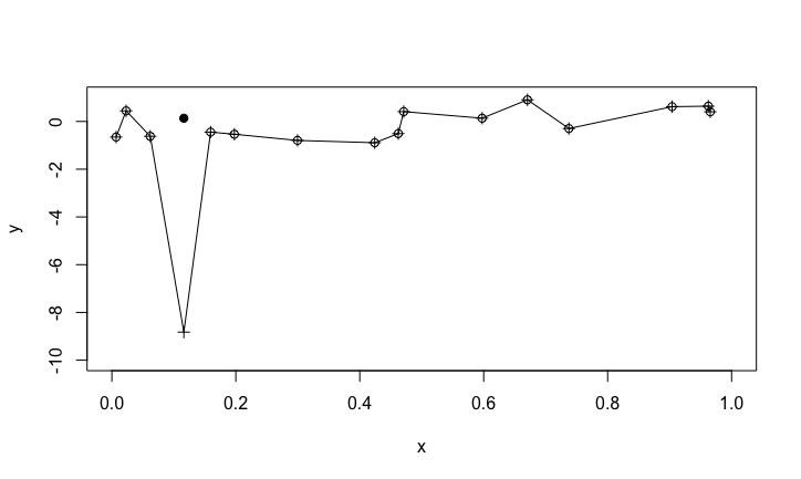
Prediction

    newx <- runif(1) 
    newy <- runif(1) # add a new data point 
    plot(c(0,1),c(-1,1), type = 'n', xlab = 'x', ylab = 'y')
    points(x,y)
    points(newx,newy, pch = 19)
    lines(sort(c(x,newx)), predict(interp, data.frame(x = sort(c(x,newx)))))
    points(sort(c(x,newx)), predict(interp, data.frame(x = sort(c(x,newx)))), pch = 3)

Prediction of a new random data point

What the polynomial really looks like

Fitted polynomial

Linear regression

    linreg <- lm(y ~ x) # linear regression
    plot(x,y)
    points(newx,newy, pch = 19)
    sx <- sort(x)
    lines(sx, predict(linreg, data.frame(x = sx)))

Linear regression of the data

The linear regression has two parameters, (intercept and slope). Between 2 and 15 parameters, there is probably a optimal number of parameters that can be fitted for a given dataset.

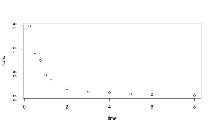
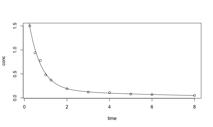
Pharmacokinetics

We use the pharmacokinetics of Indomethacin dataset Indometh from the datasets package in R.

    Indo.1 <- Indometh[Indometh$Subject == 1, ]
with(Indo.1, plot(time,conc))

Indometh dataset, patient 1

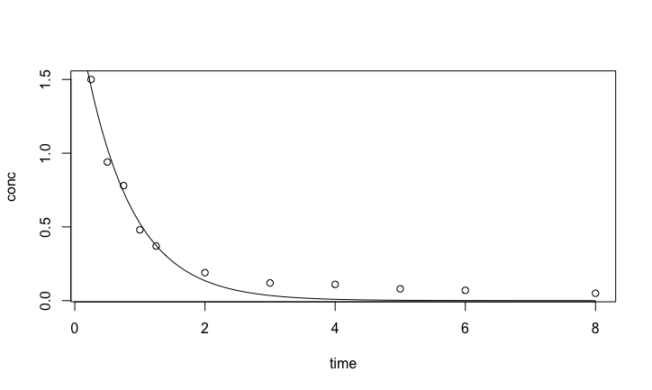
Nonlinear fit with a known model function

We perform a nonlinear least-square fit with the routine nls from R. The response variable is the concentration conc, the independent variable is time, and the model is \[ m(t) = c_0 \exp( - k t) \] with two parameters \(c_0\) and \(k\).

    indometh.nls <- nls(conc ~ c0 * exp(- k * time),  # model
    data = Indo.1,                # dataset
    start = list(c0 = 1, k = 0))  # initial guess for the parameters
    lines(seq(0,8, by = 0.1),predict(indometh.nls, list(time = seq(0,8, by = 0.1))))

Result of the nonlinear model

  Formula: conc ~ c0 * exp(-k * time)

Parameters:
   Estimate Std. Error t value Pr(>|t|)    
c0   2.0332     0.1392   14.60 1.42e-07 ***
k    1.3563     0.1232   11.01 1.60e-06 ***
---
Signif. codes:  0 '***' 0.001 '**' 0.01 '*' 0.05 '.' 0.1 ' ' 1

Residual standard error: 0.07371 on 9 degrees of freedom

Number of iterations to convergence: 10 
Achieved convergence tolerance: 8.285e-06

Result of the nonlinear model

Indometh data fitted with conc ~ c0 * exp(-k * time)

Nonlinear regression with an ODE model

To have a basis for comparison, we use the same dataset and the same model, except we express the model as an ODE

\[ \frac{dC}{dt} = - k C \] with initial condition \(C(0) = c_0\). The code is a bit more complex but the results is identical to the exponential model

    Formula: conc ~ odemodel(time, c0, k)

    Parameters:
         Estimate Std. Error t value Pr(>|t|)    
    c0   2.0332     0.1392   14.60 1.42e-07 ***
    k    1.3563     0.1232   11.01 1.60e-06 ***
    ---
    Signif. codes:  0 '***' 0.001 '**' 0.01 '*' 0.05 '.' 0.1 ' ' 1

    Residual standard error: 0.07371 on 9 degrees of freedom

    Number of iterations to convergence: 7 
    Achieved convergence tolerance: 3.348e-06

Refining and selecting a model

The fit with the exponential model is quite good at initial times, but after 2 hours, the concentration decreases more slowly than the fitted exponential. This may be because there is residual amount of drugs in peripheral tissues with slower elimination rates. A bi-exponential can take care of the two section of the pharmacokinetic data \[ b(t) = c_{01} \exp ( - k_1 t ) + c_{02} \exp( - k_2 t ) \]

Fitting the bi-exponential model

The R code is

    biexpmodel <- function(Time,c01,c02,k1,k2) {
            return(c01*exp(- k1 * Time) + c02*exp(- k2 * Time))
    }
    with(Indo.1, plot(time,conc))
    indometh.biexp <- nls(conc ~ biexpmodel(time,c01,c02,k1,k2),  # model
            data = Indo.1,                # dataset
            start = list(c01 = 2, c02 = 1, k1 = 2, k2 = 1))  # initial guess for the parameters
    lines(seq(0,8, by = 0.1),predict(indometh.biexp, list(time = seq(0,8, by = 0.1))))

Result with the bi-exponential model

Indometh data fitted with a bi-exponential

The fit looks much better! That the fit is better is to be expected, the bi-exponential includes as a subset the exponential model. So, it is really better? One way to test this is with the Akaike Information Criterion.

Akaike Information Criterion

The Akaike Information Criterion (AIC) can be used select the most appropriate model. It takes into account the SSE and the number of model parameters.

    print(c(AIC_biexp = AIC(indometh.biexp), AIC_exp = AIC(indometh.nls)))

    AIC_biexp   AIC_exp 
    -34.01319 -22.35806 

The lower the AIC, the better. Here the bi-exponential clearly wins over the exponential model.

Exercise 1

The bi-exponential model can also be expressed as the solution of a system of ODEs. How could it look likes?

Exercise 2

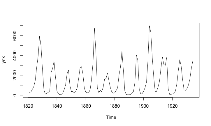
The figure shows the number of lynx in trapped in Canada between 1821 and 1934. If you were a planner, trying to manage the lynx population in a sensible way, how would you do?

Number of lynx trapped in Canada

Exercise 3

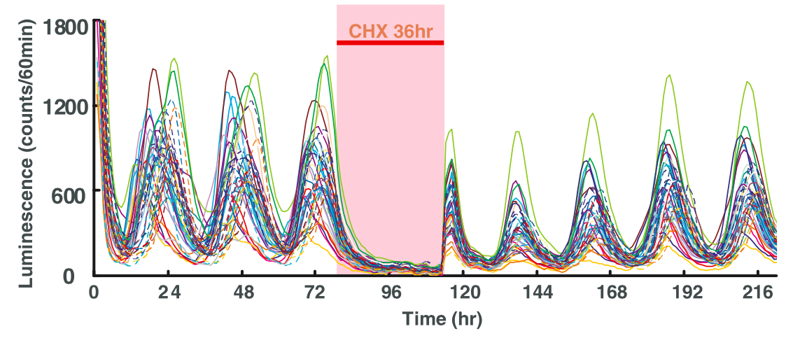
The figure shows the bioluminescence of a luciferase reporter protein with a mPer2 promoter. How would you design a mPer2 model?

Bioluminescence

References

MJ Crawley, The R Book, 2012, Wiley