Other formalisms
Other dynamical modeling formalisms include
stochastic processes
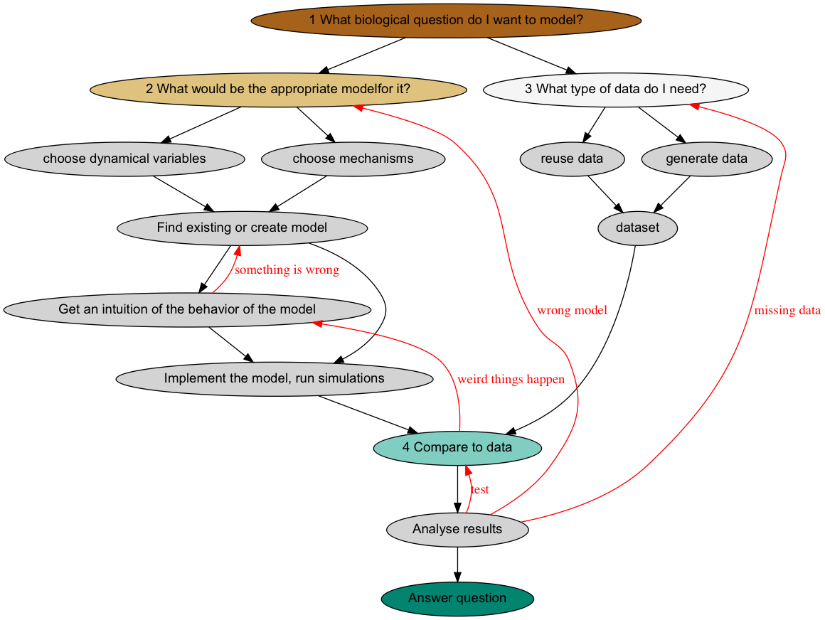
A dynamical model is a mathematical or computer model where the variables, or quantities of interest, vary in time.
difference equations
\[ \overbrace{x_{t+1}}^{\text{dynamical variable}} = \overbrace{f(x_t)}^{\text{update rule}}. \]
For example, the famous logistic map for the growth of a population with \(f(x) = x(1-x)\)
\[ x_{t+1} = \overbrace{r}^{\text{growth rate}} x_t \overbrace{( 1 - x_t )}^{\text{limiting factor}}. \]
A dynamical model is a mathematical or computer model where the variables, or quantities of interest, vary in time.
Ordinary Differential Equations
An ordinary differential equation is an equation that sets a relationship between a set of variables and their derivatives with respect to continuous independent variable (here the independent variable is time \(t\)).
\[\begin{align*} \overbrace{\frac{dx}{dt}}^{\text{rate of change}} = \overbrace{f(x)}^{\text{rule of change}}. \end{align*}\]
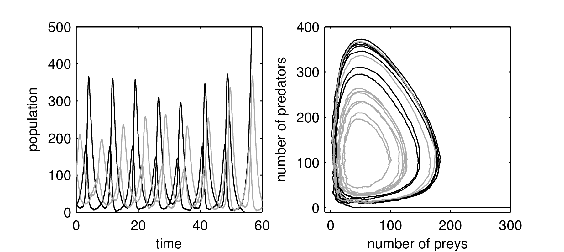
The Lotka-Volterra model was developed to study predator-prey interaction.
\[\begin{align*} \frac{dx}{dt} & = \overbrace{y x}^{\text{harvest term}} - \overbrace{a}^{\text{death rate}} x, \quad \text{predator}, \\ \frac{dy}{dt} & = \overbrace{b}^{\text{growth rate}} y - \overbrace{x y}^{\text{harvest term}}, \quad \text{prey}. \end{align*}\]
Dynamical models include dynamical variables and constant model parameters.
Logistic map \[ \color{red}{x_{t+1}} = \color{blue}{r} \color{red}{x_t} ( 1 - \color{red}{x_t} ). \]
Lotka-Volterra \[\begin{align*} \frac{d\color{red}{x}}{dt} & = \color{red}{y} \color{red}{x} - \color{blue}{a} \color{red}{x}, \\ \frac{d\color{red}{y}}{dt} & = \color{blue}{b} \color{red}{y} - \color{red}{x} \color{red}{y}. \end{align*}\]
Dynamical variables are observed quantities: gene expression, cell count, fluorescence intensity, transmembrane potential
Model parameters are determined by the biochemical, biological or physiological properties of the system: binding affinities, division rates, protein stability
Estimating parameter values given a model and experimental data is the subject of the session Inferring model parameters.
Other dynamical modeling formalisms include
stochastic processes
Other dynamical modeling formalisms include
partial differential equations
Other dynamical modeling formalisms include
individual-based models
Motifs are small blocks of regulation that can be used to distill all the complexity of biology into simple parametric term.

Linear. The species dies or is removed at a rate proportional to its level, with a constant \(k\):
\[k x.\]
Example: a protein with initial concentration \(x_0\) is degraded at a rate \(k = 0.1\) per hour, and is not synthesized. The equation for the concentration of \(x\) is
\[dx/dt = - kx,\] \[x(0) = x_0.\]
This ODE has an explicit solution \(x(t) = x_0 e^{-k t}\), the concentration decreases exponentially.
Saturated. The loss rate is linear with constant \(k_0/K\) when \(x\) is small, but saturate to a fixed value \(k_0\) when \(x\) is large
\[k_0 x/(K + x).\]
Production refers to a supply of the species that does not depend directly on its concentration
\[b.\]
Example: a protein with initial concentration \(x_0\) is degraded at a rate \(k = 0.1\) per hour, and is synthesized at a rate \(b\) per hour,
\[dx/dt = b - kx,\] \[x(0) = x_0.\]
Linear with rate constant \(r\)
\[r x\]
Logistic (competition)
\[r x ( 1 - x/K )\]
Negative feedback
\[r_0 /(K^h + x^h)\]
Positive feedback
\[r_0 x^h / (K^h + x^h)\]
Parameter \(h\) is a cooperativity coefficient, also called Hill coefficient. High Hill coefficients can lead to complex dynamics such as oscillations and bistability.
R, with the package deSolve.All major programming languages offer some numerical solvers:
matlabpythonscilaboctaveC (with the scientific library gsl)User-friendliness may vary.
Here is the simplest ODE model we can think of, the linear birth-death ODE model,
A species (e.g. mRNA, protein, drug, cell population) has
The ODE is for the concentration \(x\) of the species
\[ \frac{dx}{dt} = b + rx - kx. \]
birthDeath <- function(Time, State, Pars) {
  with(as.list(c(State, Pars)), {

    deathRate         <- k * x
    productionRate    <- b
    proliferationRate <- r * x

    dxdt     <- productionRate + proliferationRate - deathRate

    return(list(c(dxdt)))
  })
}

pars  <- c(k  = 0.5,     # per day, death rate
           b  = 0.2,     # individuals per day, production from outside source
           r  = 0.1 )    # per day proliferation (or reproduction) rate

y0  <- c(x = 1.0)
timespan <- seq(0, 20, by = 0.1)
birthDeath.sol <- ode(y0, timespan, birthDeath, pars) plot(birthDeath.sol)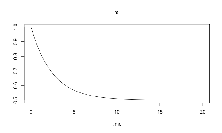
Birth/death model
Two species: preys and predators.
The prey (with density \(y\))
reproduces at a linear rate with rate constant \(b\)
\[by\]
is harvested by the predator at a linear rate with rate constant proportional to the predator density \(x\)
\[xy\]
(there is a constant 1 in front of this term)
The predator density
reproduces at the harvest rate
\[xy\]
and dies with a linear rate with constant \(a\)
\[ax\]
The two ODEs for the predator density and the prey density
\[\begin{align*} \frac{dx}{dt} & = x ( y - a ) \\ \frac{dy}{dt} & = y ( b - x) \end{align*}\]
LotkaVolterra <- function(Time, State, Pars) {
  with(as.list(c(State, Pars)), {

    killingRate       <- Prey * Predator
    preyGrowthRate    <- rGrowth * Prey
    predatorDeathRate <- rDeath * Predator

    dPreydt     <- preyGrowthRate - killingRate
    dPredatordt <- killingRate - predatorDeathRate

    return(list(c(dPreydt, dPredatordt)))
  })
}

pars  <- c(rGrowth  = 0.5,    # per day, growth rate of prey
           rDeath   = 0.2 )   # per day, death rate of predator

y0  <- c(Prey = 10, Predator = 2)
timespan <- seq(0, 200, by = 1)
LotkaVolterra.sol <- ode(y0, timespan, LotkaVolterra, pars)plot(LotkaVolterra.sol)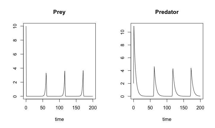
Lotka-Volterra dynamics
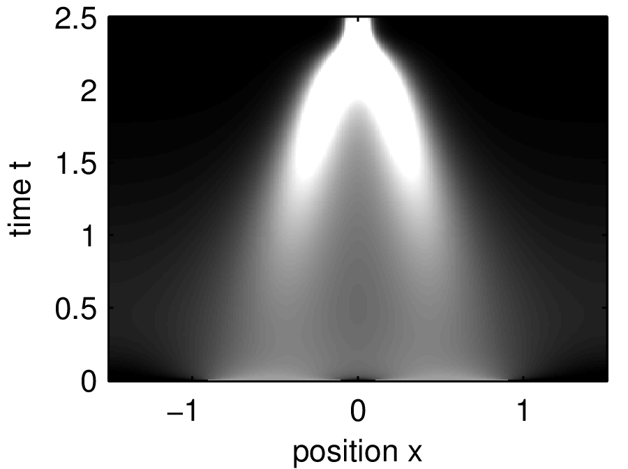
Here we take mRNA concentration \(X\), a protein product concentration \(Y\) and a modified protein complex acting as a repressor concentration \(Z\).
Degradation and production rates of the protein and the repressor are set to the value \(\beta\) and the mRNA degradation rate to \(\alpha\).
Using the negative feedback motif, we can write down the mRNA synthesis rate as
\[ f(Z) = k_0 \frac{K^h}{K^h + Z^h}. \]

Diagram of the Goodwin network. Arrow heads denote positive effect and “tee” heads denote negative effects.
We obtain a set of three ODEs \[\begin{align*} \frac{dX}{dt} & = f(Z) - \alpha X, \\ \frac{dY}{dt} & = \beta ( X - Y ), \\ \frac{dZ}{dt} & = \beta ( Y - Z ). \end{align*}\]
Goodwin <- function(Time, State, Pars) {
  with(as.list(c(State, Pars)), {

    mRNAproductionRate <- k0*K^h/(K^h + Z^h)
    mRNAdegradationRate    <- alpha * X

    dXdt <- mRNAproductionRate - mRNAdegradationRate
    dYdt <- beta * ( X - Y )
    dZdt <- beta * ( Y - Z )

    return(list(c(dXdt, dYdt, dZdt)))
  })
}

pars  <- c(k0      = 2,    # transcripts per hour, max mRNA synthesis rate
           alpha   = 1.0,  # per hour, mRNA degradation rate
           beta    = 1.0,  # per hour, kinetic rate
           K       = 1,    # mmol, half-repression concentration
           h       = 20 )  # no unit, Hill coefficient

y0  <- c(X = 1, Y = 0, Z = 0)
timespan <- seq(0, 20, by = 0.1)
Goodwin.sol <- ode(y0, timespan, Goodwin, pars)
Solution of the Goodwin model. Solutions are oscillatory.
Positive feedback loop are inherently unstable. They do occur in irreversible events such as mitosis, birth giving, differentiation and lineage choice, etc.
The positive feedback loop rests on the positive loop motif for the production of the species with concentration \(X\). \[\begin{align*} g(X) = k_0 \frac{X^h}{K^h + X^h}, \end{align*}\] where the Hill coefficient \(h > 1\).
\[ \frac{dX}{dt} = g(X) - a X. \]
Steady states: \(a X = g(X)\).
Bistability <- function(Time, State, Pars) {
  with(as.list(c(State, Pars)), {

    mRNAproductionRate <- k0*X^h/(K^h + X^h)
    mRNAdegradationRate    <- a * X

    dXdt <- mRNAproductionRate - mRNAdegradationRate

    return(list(c(dXdt)))
  })
}

pars  <- c(k0      = 2,    # transcripts per hour, max mRNA synthesis rate
           a       = 1.0,  # per hour, mRNA degradation rate
           K       = 1,    # mmol, half-repression concentration
           h       = 20 )  # no unit, Hill coefficient

y0  <- c(X = 1.1)
timespan <- seq(0, 20, by = 0.1)
Bistability.sol1 <- ode( c(X = 0.9), timespan, Bistability, pars)
Bistability.sol2 <- ode( c(X = 1.1), timespan, Bistability, pars)
Bistability.sol3 <- ode( c(X = 1.0), timespan, Bistability, pars)plot(Bistability.sol1, Bistability.sol2, Bistability.sol3)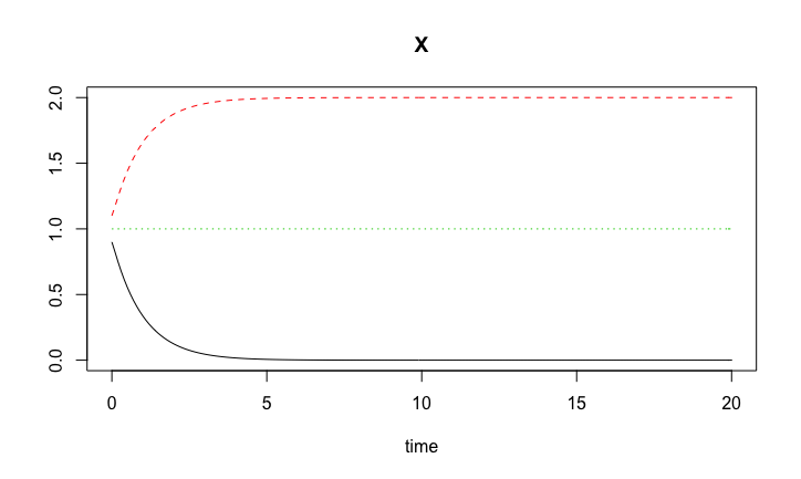
Solutions to the bistability model
The logistic map is the difference equation \[
x_{t+1} = r x_t ( 1 - x_t ),
\] for \(t=0,1,...\), with the initial condition \(x_0\) given. The R codes to solve the logistic map follow the same lines as ODE models, except that the we use the iteration method.
LogisticMap <- function(Time, State, Pars) {
  with(as.list(c(State, Pars)), {

    xiter     <- r * x * ( 1 - x )

    return(list(c(xiter)))
  })
}

pars  <- c(r  = 3.76 )     # basal growth parameter

y0  <- c(x = 0.2)
timespan <- seq(0, 50, by = 1)
LogisticMap.sol <- ode(y0, timespan, LogisticMap, pars, method = "iteration")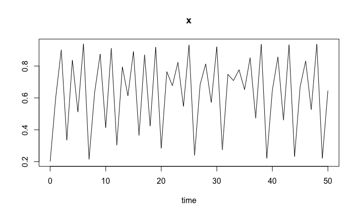
Logistic map time series
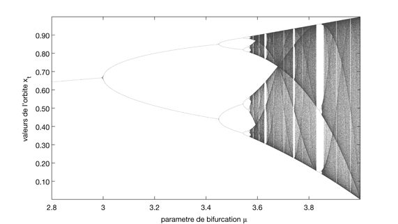
Period doubling bifurcation road to chaos in the logistic map